Google Sheets has a "Pivot table" option which allows you to create summary reports from your existing data.

In this tutorial, we'll show you how to create a basic pivot table from a list of individual order data.

The pivot table will group the data by the "Created At" column and will display the following:

1. Number of orders per day.
2. Total quantity of all line items ordered per day.
3. Average order value per day.

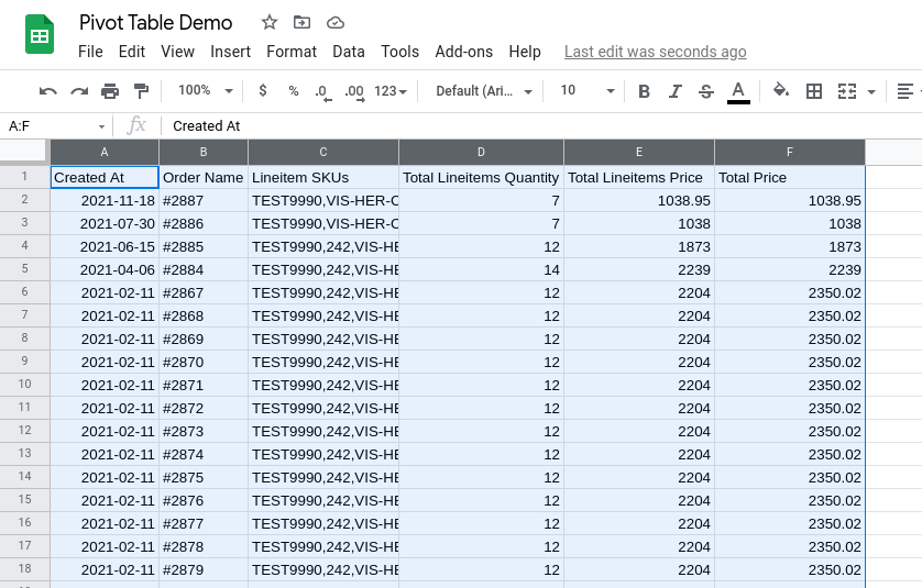
Step 1: Select the range of data to summarize.

In this example, let's select all columns.

Step 2: Click "Insert > Pivot table" from the top menu.

On the next page, choose the option "New sheet" and click the "Create" button.

Step 3: Add "Created At" to "Rows".

This is the column we want to group by.

Step 4: Add columns we want to aggregate to "Values".

For each column here, we can then specify which function to use to aggregate the values.

Step 5: Add a filter for "Created At" to hide cells with empty values.

That's it! The resulting pivot table will look something like this:

As you update values or add new rows to the source data, the pivot table gets updated automatically.